Expected_immunity

Objective:

Finding the expected immunity towards an amino acid substitution. This can hint the possibility of occurance of a mutation - When high number of people are immune to an aa_substitution over a time, then this substitution is more likely to under go a substitution/change.

Introduction:

All the mathematical models/equations used in the computation is taken from the lab's previous work.
But in lab's work x,y denotes prevalent variants of SARS_Cov2
In the present work x,y denote amino acid substitutions like "Spike_A344T", "Spike_A344A" - can be assumed like covid variant harbouring only one of the aa_substitutions.
Assumption of point 3 is followed throughout.

The Equation:

E[Immune_y(t)]=\sum_{x\in X}\sum_{s<t}\pi_x(s)\times I(s)\times P_{Neut}(t-s,x,y)

$x\in X$ :- When y is the variant of a position pos, then X is the set of all the possible variants of that position including y.
$s<t$ :- s starts from the first day of the observation period(start_date) and takes up all the values [start_date,t).
s denotes the date of infection; Here we calculate the expected immunity against variant y at time t. To do that, all possible instances of infections [start_date,t) by all possible variants of a position are considered - the double sum.
The probability of neutralisation intuitively conveys information regarding the neutralisation potential of the antibodies elicited by variant x against variant y.

Calculation of probability of neutralisation:

To calculate the probability of neutralisation by an antibody/antibodies, the probability of an antibody/antibodies binding to an variant harbouring an amino acid substituiton has to be found.
This binding probability is: $b_v(t-s,x,y)=\frac{e^{-k*[t-s]}}{FR_{x,y}(v)*IC50(v)+e^{-k*[t-s]}}$ . Where s denotes the date of occurance of the infection by variant x.
This equation is more like the pharmacokinetics equation - $\frac{concentration\space of\space ligand\_receptor\space complex}{concentration\space of\space unbound\space receptor +concentration\space of\space ligand\_receptor\space complex}$ .
Based on x and y, the values plugged in for Fold resistance differs, that is, if x=Spike_A344T, y=Spike_A344T then FR=1; else if x=Spike_A344T,y=Spike_A344A(wt) the FR>1 (taken from the table).
FR taken from a table is calculated for a position,epitope class combination. IC50 is fixed for an antibody antibody and doesn't change according to aa_substitution. Since IC50 and FR values considered here doesn't depend on the aa_substituition, $b_v(t,x,y)$ can possibly have only 2 values for a position.
In detail: In accordance to the previous point, for a position 344, on t the $b_v(t,x,y)$ for x,y combinations:- $\\ 1: \space x\neq y,\space FR_{x,y}(v)>1\\ b_v(t,s\_a344t, s\_a344a)==b_v(t,s\_a344t, s\_a344e)==b_v(t,s\_a344t, s\_a344del)\\2: \space x==y,\space FR_{x,y}(v)=1\\ b_v(t,s\_a344t, s\_a344t)==b_v(t,s\_a344e, s\_a344e)==b_v(t,s\_a344a, s\_a344a)$
So for each position, $b_v$ was found with FR>1 and with FR=1. So for each position there are two probabilitty of neutralisation values.
$P_{Neut}(t-s,x,y)=1-\prod_{v\in A}(1-b_v(t-s,x,y))$

calculating the expected immunity against a variant/aa_substitution:

$E[Immune_y(t)]=\sum_{x\in X}\sum_{s<t}\space \pi_x(s)*I(s)*P_{Neut}(t-s,x,y)$
here $\pi_x(s)$ is the frequency of variant x on day s.
$I(s)$ the incidence - Incidence reconstructed using GInPipe, data taken from Daniela.
Probability of neutralisation values are plugged in according to the x,y combination. If x==y the P_Neut for the position, calculated using FR=1 is used else the other one is used.

y=Spike\_F140I\\ X=\{Spike\_F140I,Spike\_F140F\}\\ t=03-01-2022\\ s=\{"01-01-2022","02-01-2022"\}\\ t-s=\{2,1\}\\ E[S\_f140i_{immune}(03-01-2022)]=\\ \{[\pi_{S\_f140i}(01-01-2022)*P1_{Neut}(pos=140,t-s=2)]\\+[\pi_{S\_f140i}(02-01-2022)*P1_{Neut}(pos=140,t-s=1)]\}+\\ \{[\pi_{S\_f140f}(01-01-2022)*P2_{Neut}(pos=140,t-s=2)]\\+[\pi_{S\_f140f}(02-01-2022)*P2_{Neut}(pos=140,t-s=1)]\}

This way for each variant/aa_substitution the expected immunity is calculated for everyday in the period of observation.

Algorithm of computation of expected immunity:

Function get_dis_fact:
   Pass In: start_date,end_date
   num_day=end_date-start_date
   k - is the half life
   For i=0 to num_day
     discount_factor_vector.append(round(exp(-k*i),3))
   return(discount_factor_vector)

Function get_bv:
   Pass In: fr,IC50
   Constants: start_date, End_date
   calling get_dis_fact function
   time_iter=start_date
   while(time_iter<End_date):
      days_dif=time_iter-start_date
      bv_vec.append(discount_factor_vector[days_dif]/
      (fr*IC50+discount_factor_vector[days_diff]))
      increment time_iter
   return(bv_vec)

Function Exp_immune:
   Pass In: Frequency_df,P1_neut,P2_neut, incidence
   Constant: Start_day
   For y in variants:
      For d in observation_dates:
         initialise data_frames freq_df,pneut_df,incidence_df
         dates=[start_date:d) (d not included s<t)
         dates_diff=[start_date-dates]
         For x in variants with mutation on same position as y:
            freq_df.append(Frequency_df[dates,x])
            incidence_df.append(incidence[dates])
            if y==x:
               pneut_df.append(p1[pos,dates_diff])
            elif y!=x:
               pneut_df.append(p2[pos,dates_diff])
         double_sum.sum(freq_df*pneut_df*incidence_df)
      immune_df.append(double_sum)
   return(immune_df)

All the scripts are present in "/Users/vishnushirishyamsaisundar/Documents/Master_Thesis_work/Work/Data_Analysis/Expected_immunity_computation"

Observations and modifications:

It was observed that P1(FR==1),P2(FR>1) are very similar for a position. Thats because probability of binding doesn't just depend on the FR values; Very low IC50 values can also rise the binding probability.
If one epitope classes's binding probability is higher, it can inturn increase the probaility of neutralisation of that position.
To Tackle this, for all the positions, the average IC50 (mean of all the IC50 values available in the DMS data) values were used.
Since we are not keen on the antibodies and the epitope class they belong to, average FR values for each position was computed and plugged in.
Now P_Neut becomes equal to the Binding probability, since the antibody epitope class distinction is ruled out.
Computed probability of neutralisation/binding probability with FR=1 will remain the same for all positions. So this is computed only once and then is used irrespective of position.

Unit test:

To understand the trend more intuitively, unit tests was executed.

For the Unit test purposes, the incidence is kept constant

Two positions which has high fold resistance was selected.
The temporal frequencies of the variants of these positions were assigned to deliberately induce trends
The instances of infections were combied into a date vector
In this case the summation $\sum_{s<t}$ becomes $\sum_{s\in Infec}$ , where Infec is the set of infection dates.
By tweaking the number of infections, multiple plots were obtained.
1. Only one infection that happended on the first day of the observation period 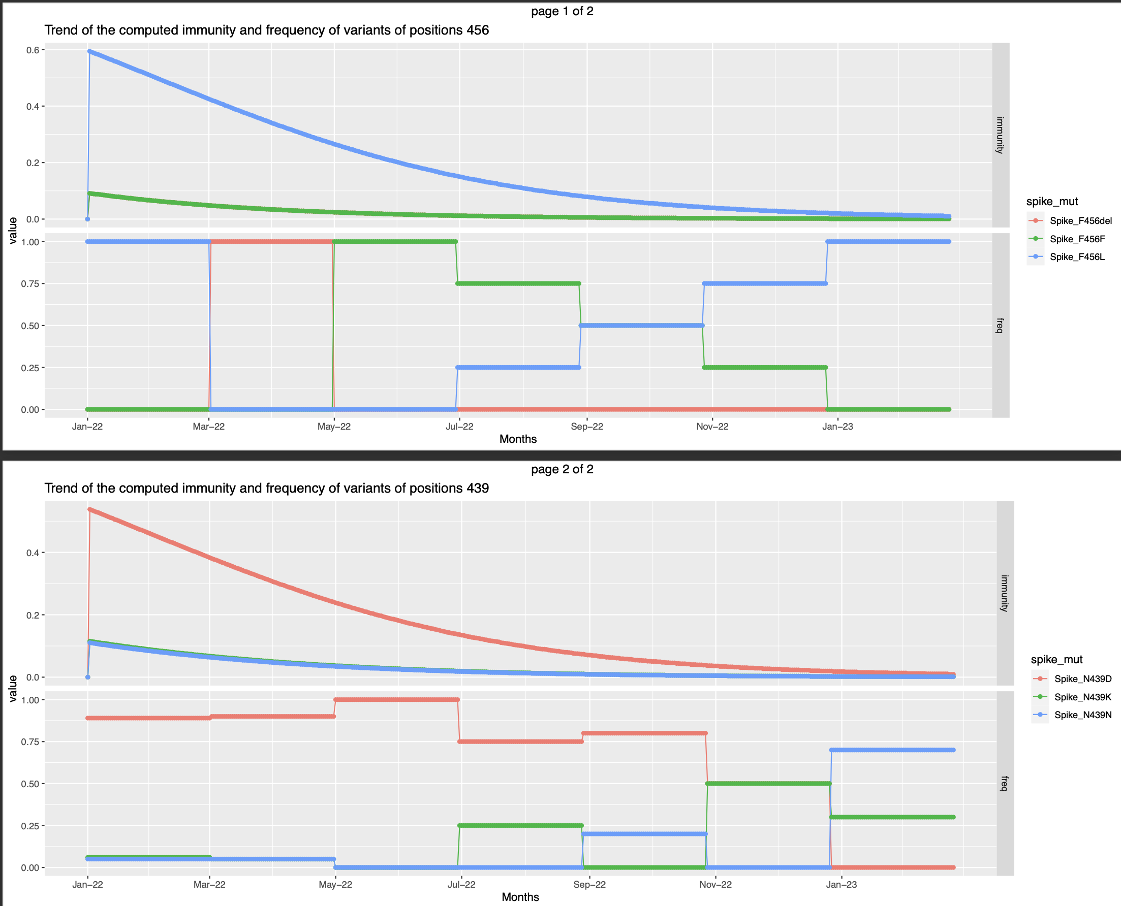The immunity is at the peak in the beginning of the observation period immediately after the infection and gradually fades away.
2. 2 instances of infection with a gap of 180 days (Jan 1,June 30) 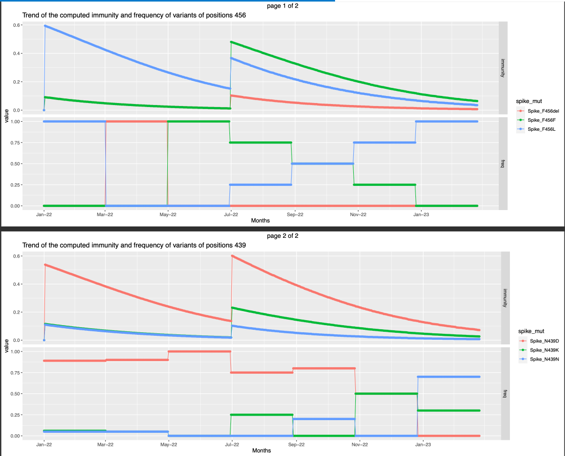Though the frequency of variant Spike_F456del is zero May22 onwards, there is a slight immunity against this variant after the second infection. This can denotes the of cross neutralisation of this variant by the infection caused by any of the other two variants.
3. Infection instances everyday from June to begining of october. The immunity against the variants gradually increases during this time period and wanes october onwards.
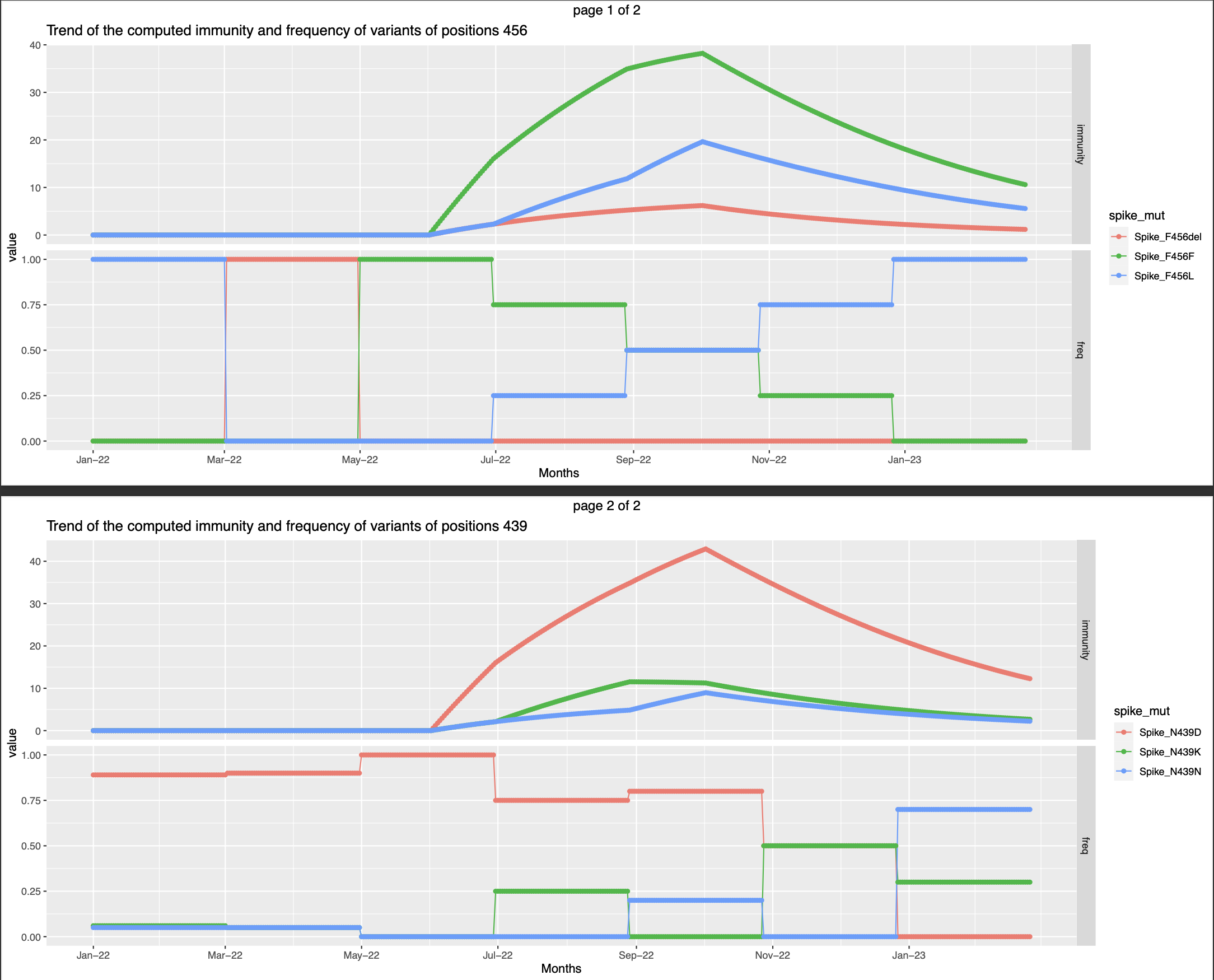
4. It is seen that the immunity is high against the variants that are abundantly present at the time of the infection . This is can also denote that that there is high probability that the infection is caused by the variant that is present abundantly and hence the immunity against it is higher in the following days.

Visualisation and analysis:

German data was used for the computation - data regarding the frequency of the variants and reconstructed incidence (data got from Daniela).
The trend of immunity is visualised along with the incidence of the mutation (incidence X frequency/proportion).
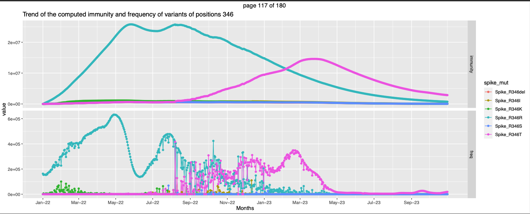
looking through each graph, there is always one variant of the position, against which the expected immunity is high. The high Numbers also doesn't vary much between positions.
Delving little further it was seen that for majority of the positions high expected immunity is against the variant which is assumed as the wild type, example: Spike_R346R is the wildt type.
HOW WAS FREQUENCY OF WILDTYPE CALCULATED:
- For a given day the frequency of all the variants of a position was calculated : $\frac{Number\space of\space times\space the\space variant\space is\space observed\space in\space the\space sequences\space collected\space on\space that\space day}{Total\space number\space of\space sequences\space collected\space on\space that\space day}$
- The frequencies of these position's variants doesn't always sum up to one. It is assumed that the $1-\sum{frequencies\space of\space the\space position's\space variants\space}$ correspond to sequences that has wildtype amino acid on the position considered.
- So for a given the position the frequency of the wild type will then be $1-\sum{frequencies\space of\space the\space positions'\space variants\space}$
For most positions this calculated frequencies of the assumed wildtype is higher than the other variants, and thats the cause of the result.
For few positions there is high expected immunity against variants that are not the assumed wildtype variant.
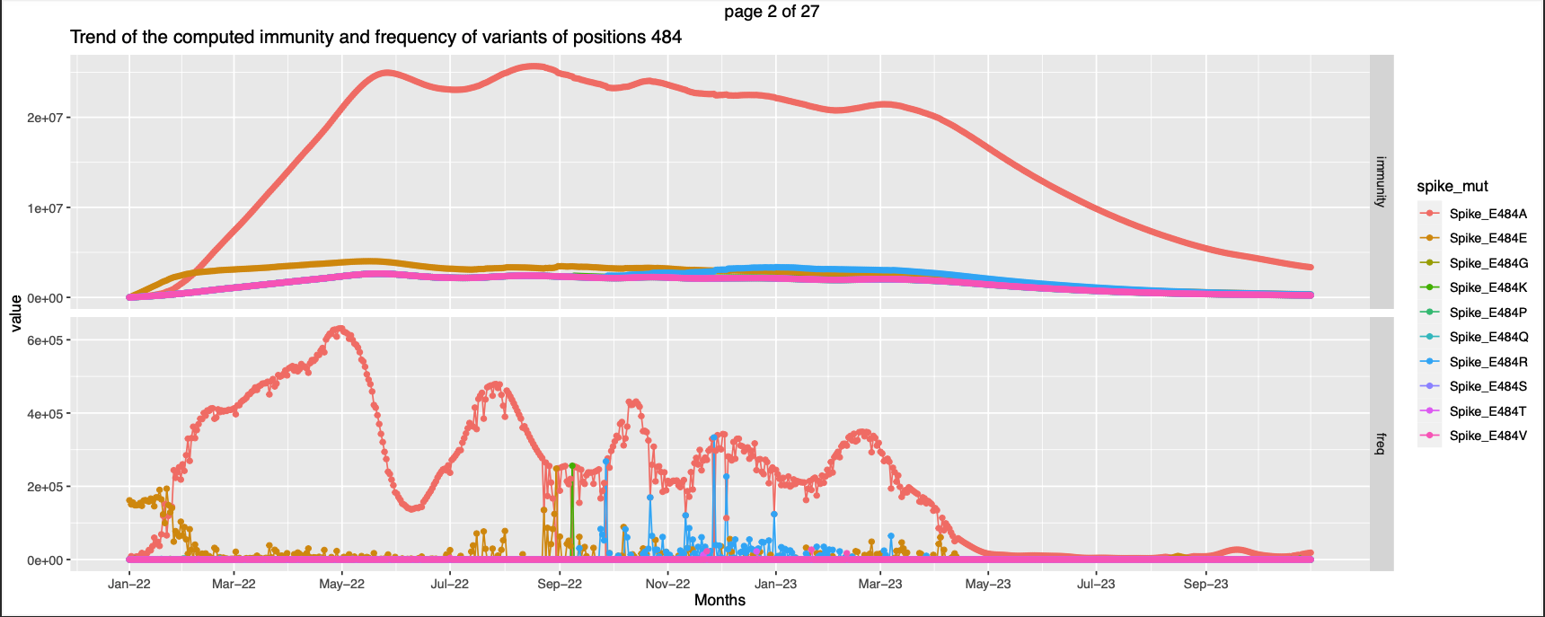
For few other positions the expected immunity against the Wild-type becomes lesser than the expected immunity against a non-wild type at somepoint in the observation period like .
These seemed interesting.

Position wise analysis

The following table holds information about only those positions which flagged as exposed by any one of the tools used, present in the screenshot provided by Max and also is present in the list of characteristic mutation positions(80% prevalance). Bigger table with all the positions is present in the excel.

Position	Significance	Trend type
19		high exp immunity against non-wt
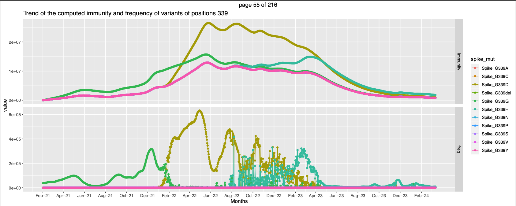
339		high exp immunity against non-wt
346		High immunity against wt and non wt at different points of time
371		high exp immunity against non-wt
373		high exp immunity against non-wt
375		high exp immunity against non-wt
376		high exp immunity against non-wt
405		high exp immunity against non-wt
408		high exp immunity against non-wt
417	Tight Binding of SARS-Cov2 with ACE2	high exp immunity against non-wt
440		high exp immunity against non-wt
446	Hydrogen bonding with ACE2	High immunity against wt and non wt at different points of time
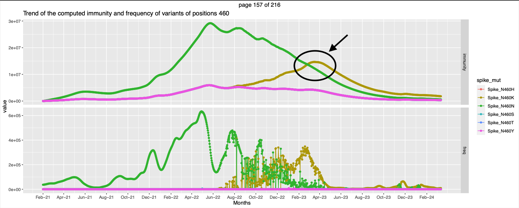
460		High immunity against wt and non wt at different points of time
477		High exp immunity against non-wt
478		high exp immunity against non-wt
484		high exp immunity against non-wt
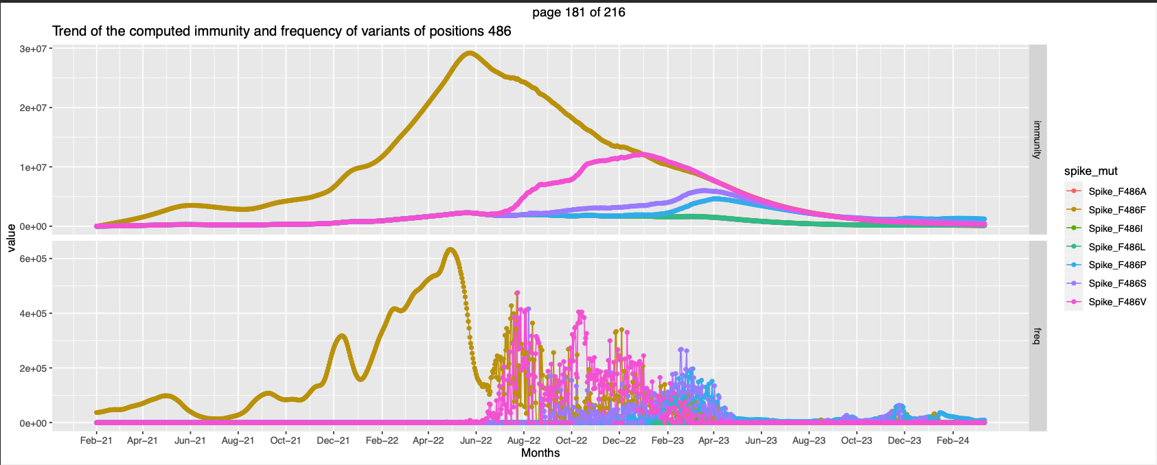
486	Tight Binding of SARS-Cov2 with ACE2	High immunity against wt and non wt at different points of time
498	Tight Binding of SARS-Cov2 with ACE2	high exp immunity against non-wt
501	Tight Binding of SARS-Cov2 with ACE2	high exp immunity against non-wt
505		high exp immunity against non-wt
157		high exp immunity against wt
158		high exp immunity against wt
245		high exp immunity against wt
252		high exp immunity against wt
356		high exp immunity against wt
403		high exp immunity against wt
445		high exp immunity against wt
450		high exp immunity against wt
456	Tight Binding of SARS-Cov2 with ACE2	high exp immunity against wt
481		high exp immunity against wt
490		high exp immunity against wt

Downside:

There is overplotting in the plots generated like in .
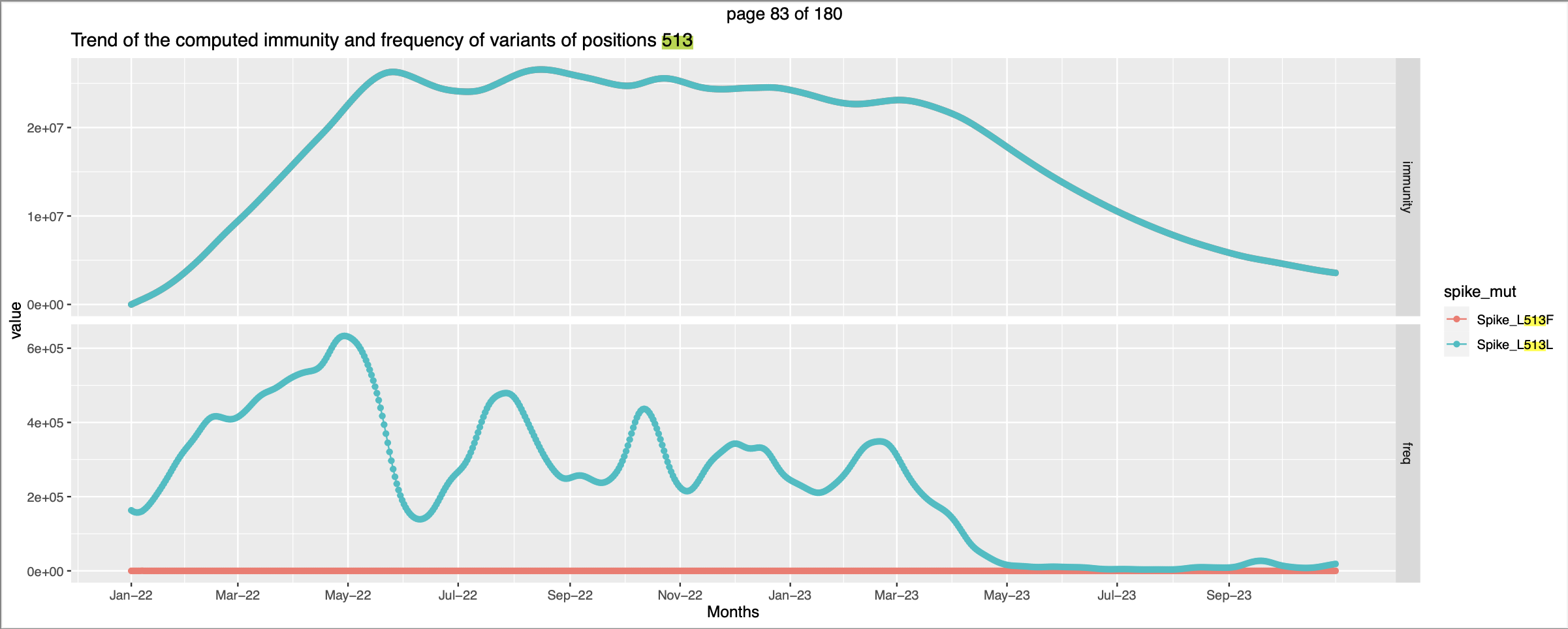Both the variants have similar expected immunity numbers, but this is not well represented by the plot
Similarly for many positions, variants that have similar expected immunity numbers are not well represented.
options like alpha, position_dodge were tried, but still couldn't deal with overplotting.

Extending to analyse trends other countries:

The analysis was repeated for 5 other countries for which the incidence and the frequency data is in hands for observation period "2022-01-01" to "2023-10-31"
It was seen that the screenshot shared by Max is indeed from the outbreakinfo site - mutation profile for 3 variants.
So including this data is like repeating the characteristic mutations condition twice. Hence the column "Present in Max's screenshot" is omitted.
So in total there are 40 positions that have been flagged as exposed by atleast one tool and is present in the list of characteristic(80% prevalance) mutations.
On analysis it was seen that the mutation against which the expected immunity is high is same in all the countries.
Definitely the numbers and the trend differs in the countries.
To have high expected immunity against same mutation in all the countries means that the frequency of the mutations is similar in all the countries.
Next step is to see how the trends of these positions go in the further data.

Extending observation period:

The reconstructed incidence is available until 2024 only for Germany. For other coutries the observation period is just exteded by few weeks.
Nevertheless the expected immunity is being computed for all the six countries for the period incidence is available.
Extending the time horizon in the forward direction is not fruitful because the frrequency and incidence are very low and so is the expecteed immunity. Not much can be derived from this.
The incidence is
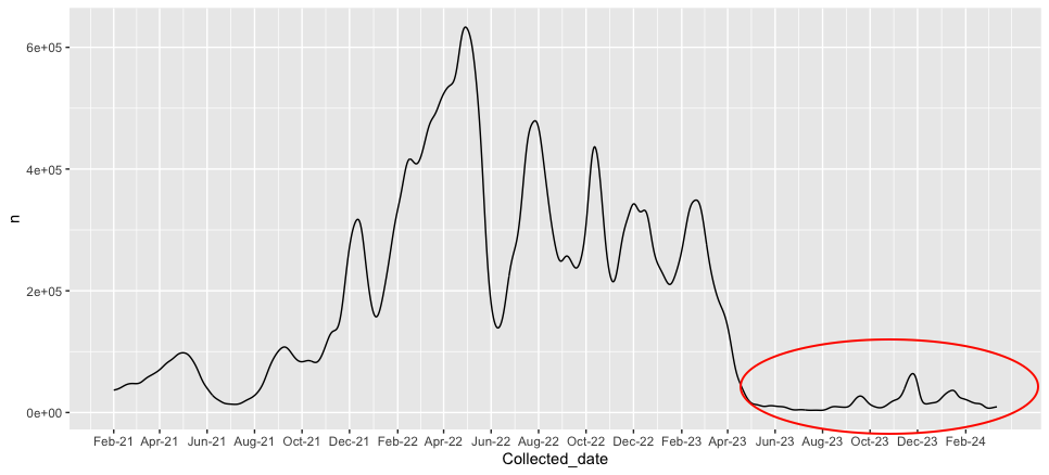
The expected immunity trend is
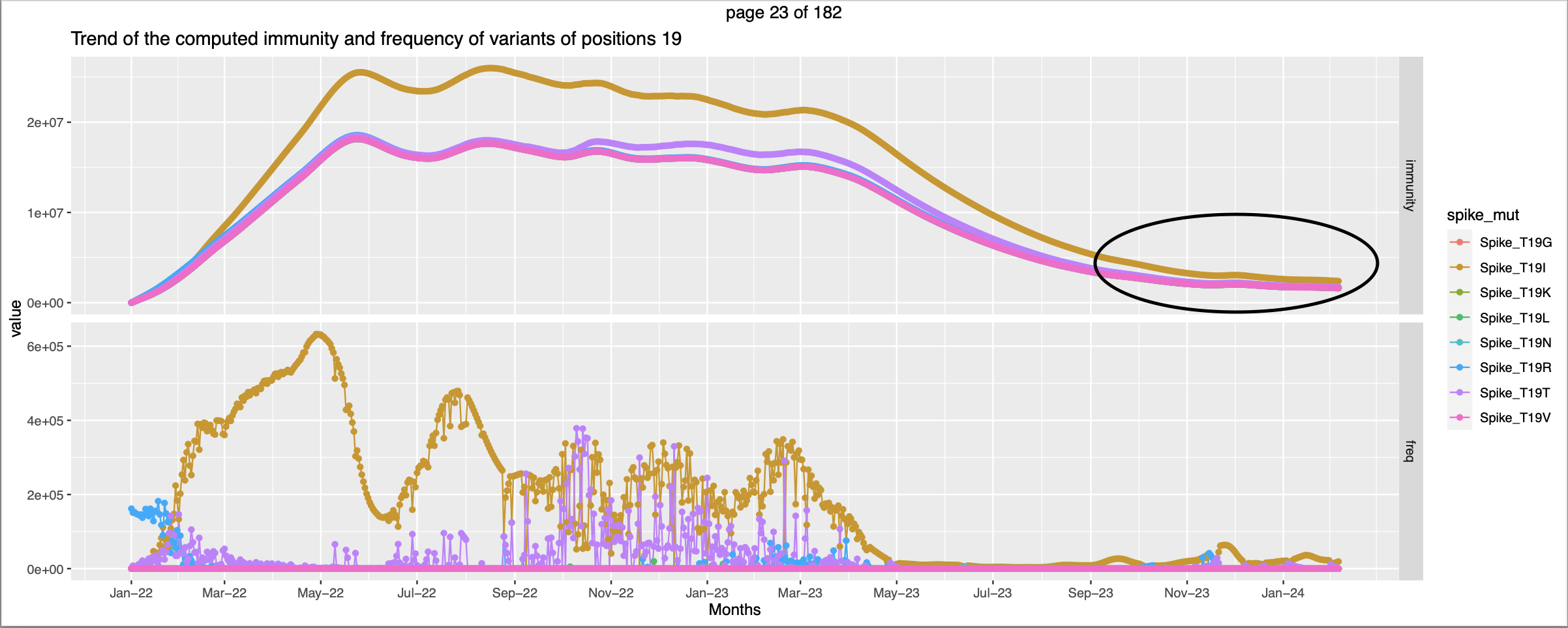
It would be good is the extension is reeterograde
For this we need daily incidence data

Trying with GInPipe:

To get daily incidence data for these countries, WHO COVID-19 dashbboard, our world in data were searched. I was able to get the weekly number of cases but not daily case numbers.
Using few epidemiological models, few groups have estimated daily case numbers and this is availale to download from Our world in Data. But the data is available only till beginning of 2021.
Looking into countries waste water surveillance dashboard - the data is about the viral load. I am not sure how to get the incidence from this.
Since I have got the aminoacid substitution data, trying out with the GInPipe is a feasible idea.
For Germany, I have got the recostructed incidence data from begining of 2021 to 2024 (data from Daniela)
For the remaining countries, I need to have the daily reported cases to get the min_incidence from GinPipe.
For this I have interpolated the weekly numbers from WHO data. The Weekly new cases numbers from OWID and WHO is the same (cross checked).
I was able to get the recostructed incidence for all the six countries (including germany)
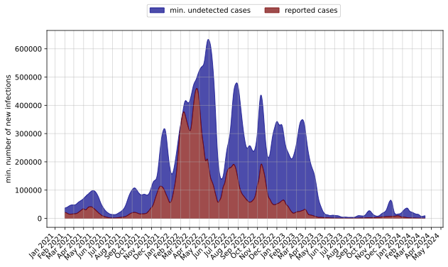
When comparing the numbers pertaining to Germany - Daniela's data vs my reconstructed one there is a huge difference. The following is the plot from Daniela's GInPipe results
The following is from my GInPipe Results
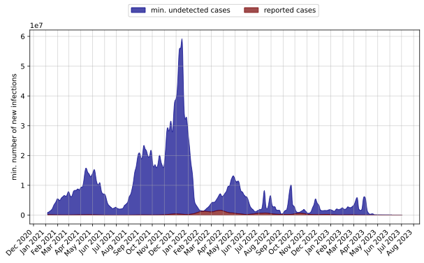
The plot of the reported cases also differ. I should cross check it before proceeding further.
Also the GInPipe parameters. I ran the pipeline with default settings.

Full data expected immunity estimation for germany:

The expected immunity (2021 - 2024) is calculated for Germany (using Daniela's incidence data)
plots of 40 Positions (positions that has 80% mutation prevalance in all the variants and has been flagged as exposed by atleast one of the 3 tools) were first taken.
Out of this 40 plots, plots that has trends of 2 mutations doing a crossover was alone selected
This brings the number to 22 positions.
There are common expected immunity trend among the positions
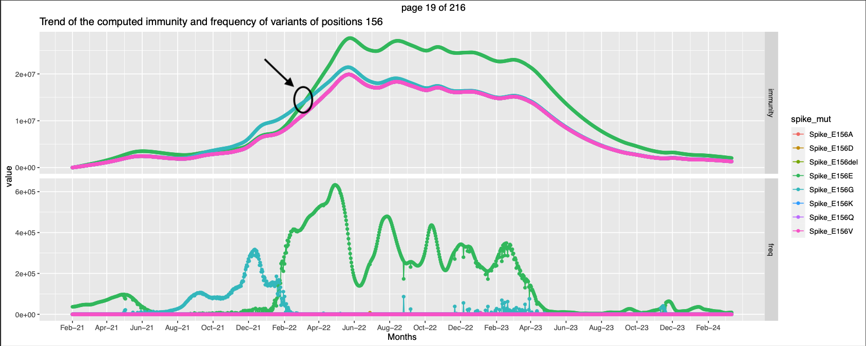
For positions 19,156,157,158, there is an instance of small crossover between the exp immunity trend against 2 mutations.
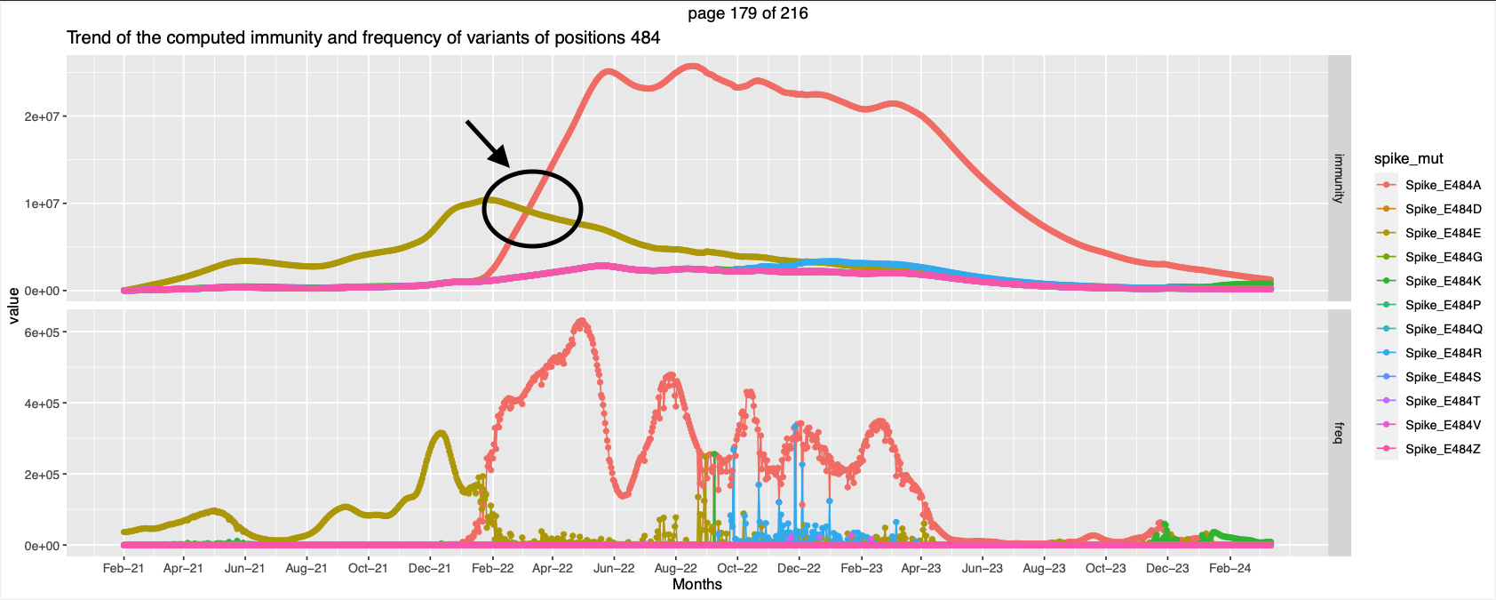
For Positions 371, 373, 375, 376, 405,408, 417, 440,477, 484, 498, 505, 501 has apparent crossover. With a small peak preceding the crossover.
Positions 346, 446, 460, Peak in immunity against a different mutation while the immunity trend of the former goes down.
Position 339 there is an initial crossover between two mutations and also a partial overlapping between two other mutations at the end.
Position 486 has peaks of other muatations when the peak of Spike_F486F goes down. It seems like there is similar expected immunity against atleast 4 different mutations. .

What can a crossover in the trend mean?

The crossover seen in the plots involves exp immunity trends against different mutations, one of the two trend traces a decline while other is in an increasing trend. In the case of the light cross over, both the trends are on increase, but the rise of one trend is sharper than the other.
These crossover can imply that occurance of a one mutation is declining while the other is increasing - the occurance of a mutation is favoured over the other. Higher the occurance, higher is the expected immunity agaist it.

Possible questions:

Why at certain positions the occurance of the wt residue is always higher than other possible variants? How important are these residues for the function of the protein?